This is the first blog that documents the coding period of my GSoC21 journey. I learned a few exciting things in these two weeks, as I expected I would. So, let’s dive in and see if you knew a few of this stuff I learned.

Starting off !!!

I started by getting a brief idea of the scope of the changes that could be done to the data frame. This was the task I had decided on for the first week. Whenever we are involved in a project that runs for anywhere between 2-4 months, it is essential to have a timeline or a roadmap of sorts to look back to. This doesn’t have to be something rigid. We can choose to deviate from it, and in fact, deviations are bound to happen due to multiple reasons. It can happen because of an unexpected bug in between, or because you came across some alternative that you did not consider initially, or simply because it is one of those projects that gives better insights as you dwell into it.

Every good GSoC proposal consists of a tentative timeline that depicts the work we plan on doing as the weeks progress. Here is the timeline I had submitted in my proposal.

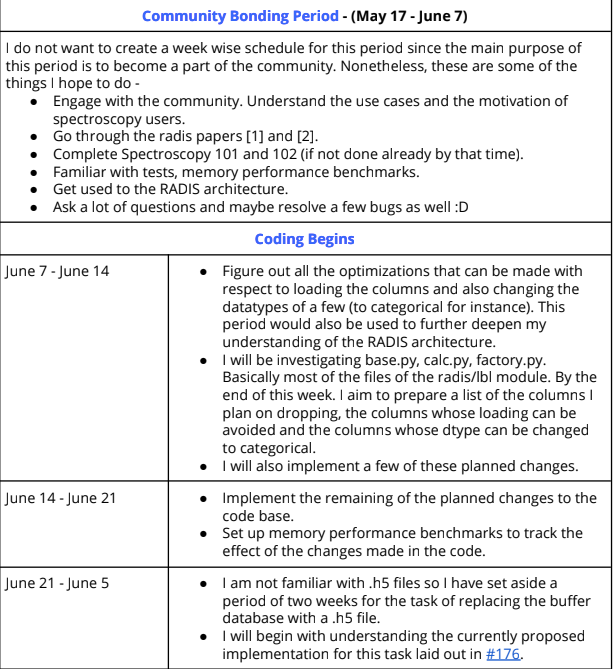
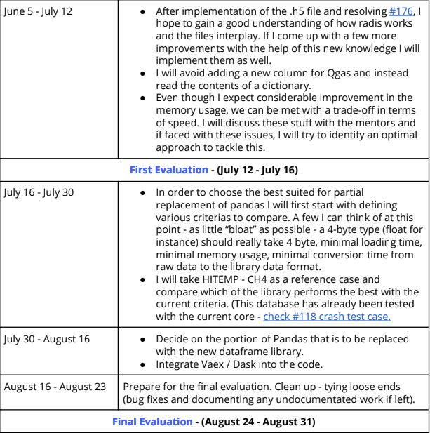
So as per this, I was supposed to finish off the refactors to the data frame and finish setting up the benchmarks. But I was unable to complete these. I had underestimated the work it would take to achieve them. Nonetheless, I also did have some time to look up the things I am supposed to do in the second half of the coding period.

Memory and Time performance benchmarks - Tic-Tok

Before making any changes to the codebase, Erwan suggested I have the benchmarks setup. So what do I mean by this? To make sure that the changes I am making to the code are indeed reducing the computations’ memory consumption, we use a few tools that help us track the memory consumption for various calculations as a function of git commits. Multiple tools help us do this. Radis already used a tool developed by airspeed velocity to track the memory computations. I ran into many troubles in setting these up, and I lost a lot of valuable time in the process. Ultimately, Erwan fixed it, and I was able to run the benchmarks on my machine.

The benchmarks still seem to take a lot of time to run through, and for them to be feasible to be used as a tool through which I can check the performance regularly, I need to learn a few things. I hope to pick these up in the next few days.

We are also trying to look at a few other alternatives that we can use instead of asv. I will update you guys regarding this in the next blog post.

Oh Pandas here I deal with you !

Let’s ditch a few columns

We can reduce the memory usage of pandas by using one straightforward trick - avoid giving loading the columns that are not required for computation. Below I demonstrate how just dropping a few columns can provide significant improvement in memory consumption. I am using the HITEMP-CH4 database for demonstration.

 1
 2
 3
 4
 5
 6
 7
 8
 9
10

>>> from radis.io.hitran import hit2df
>>> df = hit2df("06_HITEMP2020_2000.0-2500.0.par")
...
>>> df.info(verbose=False, memory_usage="deep")
...
memory usage: 30.5 MB
>>> df.drop(["id", "iso"], inplace=True, axis=1)
>>> df.info(verbose=False, memory_usage="deep")
...
memory usage: 25.4 MB

The peak memory usage before dropping the columns was 30.5 MB, and once I remove a few columns, the peak memory usage becomes 25.4 MB. I have already implemented the dropping of the id column and handled the case of a single isotope by dropping the column and instead just storing the isotope information as a meta attribute. We have also finalized the discarding of the other columns by considering the physics of these quantities. Let’s check out a few of them. Since I haven’t already implemented the optimizations that follow, I will save the implementation details for the next blog.

Einstein’s Coeffecients and Linestrengths

There are four parameters of interest to describe the intensity of a line : Linestrength $(int)$, Einstein emission coefficient $(A)$ and Einstein absorption coefficient $(B_{lu})$, Einstein induced emission coefficient $(B_{ul})$. All of them are somehow linked to the Squared Transition Dipole Moment $(R)$. ¹

$$ S(T) = S_0 \frac{Q_{ref}}{Q_{gas}} \operatorname{exp}\left(-E_l \left(\frac{1}{T_{gas}}-\frac{1}{T_{ref}}\right)\right) \frac{1-\operatorname{exp}\left(\frac{-\omega_0}{Tgas}\right)}{1-\operatorname{exp}\left(\frac{-\omega_0}{T_{ref}}\right)} $$
$$ B_{lu}=10^{-36}\cdot\frac{8{\pi}^3}{3h^2} R_s^2 \cdot 10^{-7} $$
$$ B_{ul}=10^{-36}\cdot\frac{8{\pi}^3}{3h^2} \frac{gl}{gu} R_s^2 \cdot 10^{-7} $$
$$ A_{ul}=10^{-36}\cdot\frac{\frac{64{\pi}^4}{3h} {\nu}^3 gl}{gu} R_s^2 $$

NOTE: For a detailed explanation of all the quantities in the equation do check the reference

So now the idea would be to drop the $int$ column and use $A_{ul}$ to calculate the value of $int$ from it. The reason to drop $int$ and not $A_{ul}$ some databases like ExoMol databases only provide the value of $A_{ul}$.

Concat better

For anyone who wants to concat multiple data files, pandas tends to become useless as the memory scales up. I started experimenting with concat operations to cluster the isotopes of each type, run computations on them, and later concat them. But I later learned that since this data is already in the form of a single dataframe, indexing is a better parameter to track the memory consumption. Nonetheless, there are a few other places in Radis where we process multiple files and concat them. Hence this experiment would help us decide how to replace the current approach with a better one. I tried out three methods. I was using some random dummy data files of around 780 MBs.

• Normal pandas.concat
• Concat with a doubly ended queue
• Concat with parquet

Here are the results of each of these methods -

CPU Time - 0:02:43.797588
Peak Memory Usage - 4.1050 GB

CPU Time - 0:02:34.484612
Peak Memory Usage - 3.7725 GB

CPU Time - 0:01:37.984875
Peak Memory Usage - 1.6829 GB

Looking at the results, parquet seems like a perfect option to me. But we will run for a few more examples and later check which one suits them best. The complete code to run this experiment can be found here.

The next two weeks

I will first focus on completing the task list of the PR I created. I will start with setting up a proof-of-concept for handling molar_mass, Qgas and abundance quantities. I might require the whole week to finish this off. Once this is done I will take up #176.